Kaggle: Lyft Motion Prediction for Autonomous Vehicles
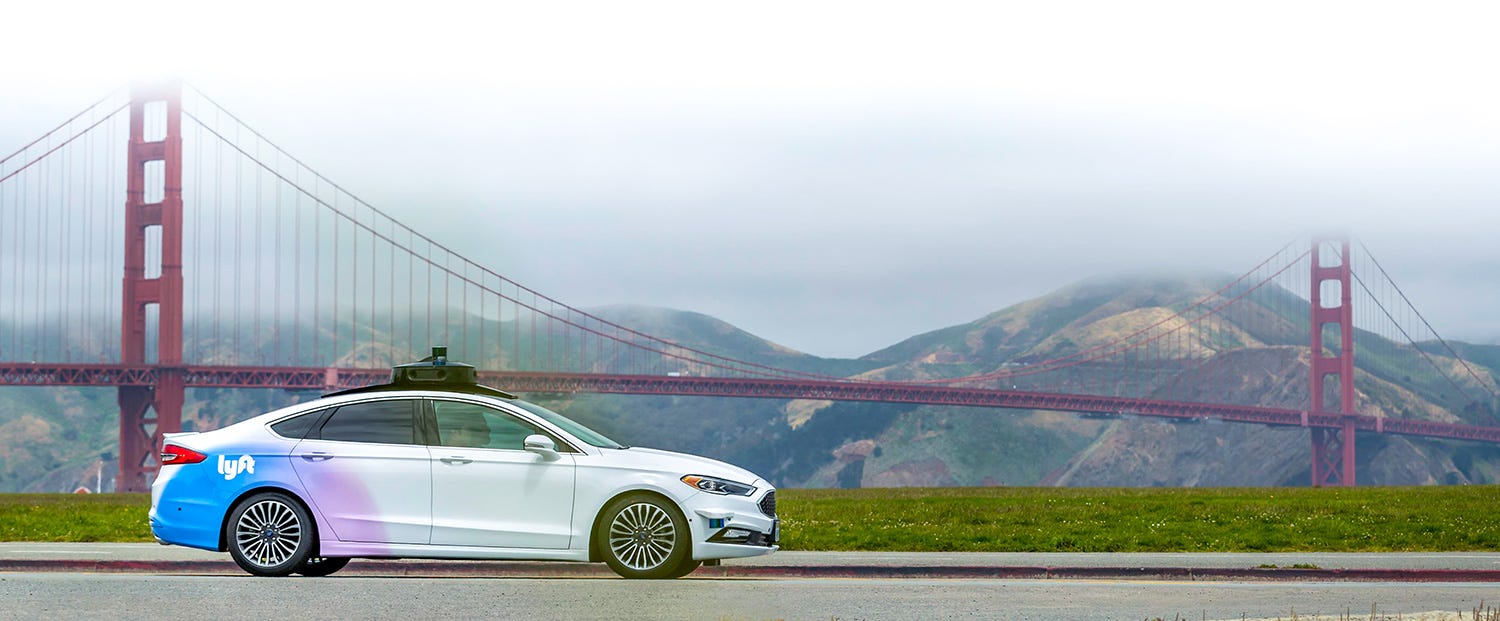
In this Kaggle competition, I built motion prediction models for self-driving vehicles to predict how cars, cyclists, and pedestrians move in the autonomous vehicles (AV’s) environment, with the support of the largest Prediction Dataset [1] ever released to train and test the models.
Competition Description

In summary, the goal of this competition is to predict other car / cyclist / pedestrian (called “agent”)’s motion in the next 5 seconds future with some past frames, based on the view of the AV’s views. A raster generates a bird’s eye view (BEV) top-down raster, which encodes all agents and the map. The network infers the future coordinates of the agent-based upon this raster.
Lyft Level 5 Prediction Dataset
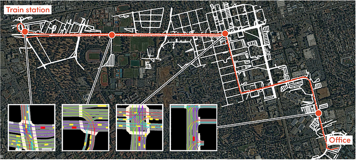
The dataset was collected along a fixed route in Palo Alto, California. It consists of 170,000 scenes capturing the environment around the autonomous vehicle. Each scene encodes the state of the vehicle’s surroundings at a given point in time.
The dataset consists of frames and agent states. A frame is a snapshot in time, consisting of ego pose, time, and multiple agent states. Each agent state describes the position, orientation, bounds, and type.

A detailed exploratory data analysis is available in this Jupiter Notebook.
Evaluation & Score
This is a brief summary of the evaluation, please refer to the metrics page in the L5Kit repository
After the positions of a trajectory are predicted, a negative log-likelihood of the ground truth data given these multi-modal predictions is calculated. Assume the ground truth positions of a sample trajectory are

and the predicted K hypotheses, represented by means

for each hypothesis, the model also generates a confidence value c (i.e. for a single model, the value c is 1). Assume the ground truth positions to be modeled by a mixture of multi-dimensional independent Normal distributions over time. The goal is to maximize the following likelihood

As for yielding the loss, we simply take the log and take the negative of the likelihood equation.


For numeral stability (preventing the condition of underflow caused by an extremely small value), the log-sum-exp trick is applied to the equation.

A huge thanks to the competition host for providing the implementation of this loss function.
Image Raster & Pixel Size Selection
In general, it is less feasible to implement and train state-of-art models for motion prediction in just 2 months. Instead, playing with the input data and applying feature engineering to them wisely is the key to winning the competition.
In this competition, the key factors for gaining higher accuracy are the image raster size the pixel size.
- raster size: the image size in pixel
- pixel size: spatial resolution (meters/pixel)
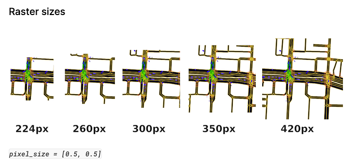
For a fixed pixel size, a larger raster size means more surrounding information. In the meantime, it also means a longer training period (more computation).

For a fixed raster size, a smaller pixel size means higher resolution.
Models
I’ve tried several baseline models. Each model has been trained for roughly 3 days on a Tesla V100 GPU. The following is a summary of the performance.
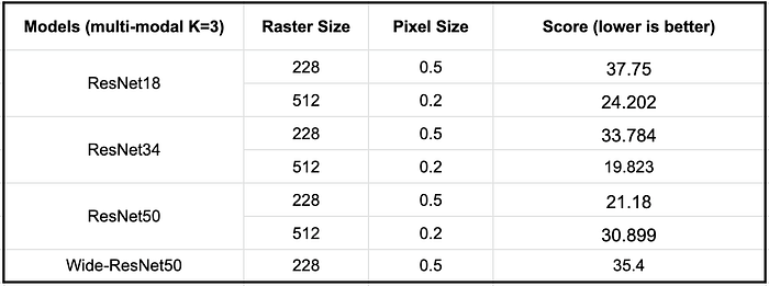
It turns out that more layers are not necessarily mean better scores. The trade-off between model/input size and the training speed further restricts my model choices. I decided to explore deeper with the models ResNet18 and ResNet34.
Ensemble
In the end, I finished the competition with a score of 19.02 in the private leaderboard and 18.938 in the public leaderboard, ranked at 94/937.
The private leaderboard is calculated with approximately 50% of the test data.
The ensembling improved my score (the best single model score) from 19.823 to 18.938 with the following models, the ensemble weights are based on their scores:
[(sum score — individual score) / (sum score * 3)]
- ResNet34 / Raster Size 512 / Pixel Size 0.2
- ResNet34 / Raster Size 350 / Pixel Size 0.4
- ResNet18 / Raster Size 512 / Pixel Size 0.2
- ResNet18 / Raster Size 448 / Pixel Size 0.3
Summary of Some Great Insights from the Top Rankers
- Ensemble with Gaussian Mixture Model (GMM).
At the final ensemble stage, GMM with 3 components was used to fit the multiple trajectory positions generated by the trained models.
- Rasterizing based on the agent’s speed.
Slow agent speed means the prediction only needs a small raster size (since the vehicle probably won’t travel too far in the next 5 seconds). In the meantime, the “slow model” increases the number of history frames to increase accuracy. Similarly, the “fast model” increases the raster size and reduces the frames.
- Extract meta-data from the Agent-Dataset
There is some useful information in the agent dataset, such as centroid, rotation, velocity, etc. A second head with two fully connected layers could be used to encode this information, and then concatenate the output vector to the output of the ResNet pooling layer.
My Experiments that Didn’t Work
- Lane encoder
I separately trained a Conv2d-Autoencoder on the semantic lane channels, and then fine-tuned with the ResNet model.
- GRU over time-stacked models
- Adding more layers on top of the ResNet head
- Graph Convolutional Network on the lane nodes
I treated each 4x4 grid in the lane map as a single node and set up the adjacency matrix based on their pixel values. (e.g., a 4x4 grid has a maximum of 8 neighbors, exclude the neighbor if the value is below a threshold, which means no lane).
Conclusion
This is my first Kaggle competition experience. It’s really encouraging to see my effort in the past three months earned a bronze medal. Also, I saw many novel usages of traditional machine learning techniques that showed their outstanding performance. My journey on Kaggle has just started.
Reference
[1] Houston, J. and Zuidhof, G. and Bergamini, L. and Ye, Y. and Jain, A. and Omari, S. and Iglovikov, V. and Ondruska, P., One Thousand and One Hours: Self-driving Motion Prediction Dataset, arXiv:2006.14480v2, 2020
